Friday, January 26, 2018

CFP Review Ratings

Introduction


We recently completed the bsides Nashville CFP. (Thank you all who submitted.  Accepts and rejects will be out shortly.)  We had 53 talks for roughly 15 slots so it was a tough job.  I sympathize with the conferences that have in the 100's or 1,000's of submissions.

CFP Scoring


Our CFP tool provides the ability to rate talks from 1 to 5 on both content and applicability.  However, I've never been happy with how it condenses this down to a single number across all ratings.

Our best guess is it simply averages all the values of both types together.  Such ratings would look like this:
(We've removed the titles as this blog is not meant to reflect on any specific talk.)

This gives us _a_ number (the same way a physician friend of mine used to say ear-thermometers give you _a_ temperature) but is it a useful one?

First, let's use the mean instead of the median:
The nice thing about the median is it limits the effect of ratings that are way out of line.  In many of our talks, one person dislikes it for some reason and gives it a substantially lower rating than everyone else.  We see talks like 13 shoot up significantly.  It also can cause drops such as talk 51.

Scoring with a little R


But what really would be helpful is to see _all_ the ratings:
Here we can see all of the ratings broken out.  It's more complex but it gives us a better idea of what is actually happening for any one talk.  The green dot is the median for all ratings combined.  The red dots are the talks' median value.  And the grey dots are individual ratings.

We can look at 13 and see it scored basically all 5's except for for one 4 in applicability, 1 'average' rating, and one below average rating bringing the median up to 5-5.  When we look at 51, we see how it had a few slightly-below-average ratings and several below-average on content, and several below-average on both content and applicability.  We also get to compare to the mean of all talks (which is actually 4-4) rather than assuming 3-3 is average for a talk.

One I find particularly interesting is 29.  It scored average on applicability, but it's content score, which we would want to be consistently high, is spread from 1 to 4.  Not a good sign.  In the first figure, it scored a 3.2 (above average if we assume 3 is average since no average is shown).  In the median figure,  it is 3.  But in this view we can see there are significant content concerns about this talk.

Conclusion


Ultimately, we used this chart to quickly identify the talks that were above or below the mean for both content and applicability.  This let us focus our time on the talks that were near the middle and gave us additional information, in addition to the speaker's proposal and our comments, to make our decision on.  If you'd like to look at the code for the figures, you can see the jupyter notebook HERE.

Future Work


In the future I could see boiling this down to a few basic scores: content_percentile, applicability_percentile, content_score range, and applicability_score range as a quick way to automate initial scoring.  We could easily write heuristics indicating that we want content ratings to meet a certain threshold and be tightly grouped as well as set a minimum threshold for applicability.  This would let us more quickly zero in on the talks we want, (and might help larger conferences as well).

Sunday, January 7, 2018

Smaller Graphs for Easier Viewing

Introduction

As I suggested in my previous blog,  visualizing graphs is hard.  In the previous blog I took the approach of using a few visual tricks to display graph information in roughly sequential manner.  Another option is to convert the graph to a hierarchical display.  This is easy if you have a tree as hierarchical clustering or maximal entropy trees will do.

Maximal Entropy Graphs

However, our data is rarely hierarchical and so I've attempted to extend maximal entropy trees to graphs.  First, it starts with the assumption that some type of weight exists for the nodes.  However, this can simply be uniform across all nodes.  This weight is effectively the amount of information the node contains.  As in the last blog, this could be scored relative to a specific node in the graph or about any other way. It then combines nodes along edges, attempting to minimize the amount of information contained in any aggregated node.  It continues this approach until it gets to the desired number of nodes, however it keeps a history of every change so that any node can be de-aggregated.

You can find the code in this Github GIST.  You can then try it out in This Jupyter Notebook.

Ultimately, it takes a graph like this:


and produces one that looks like this:

Each node still contains all the information about the nodes and edges it aggregates.  This allows an application to dig down into a node as necessary.

Future Work

Obviously there's a lot to do.  This is less a product in and of itself than a piece for making other graph tools more useful.  As such, I should probably wrap the algorithm in a visualization application that would allow calculating per-node scores as well as diving in and out of the sub-graphs contained by each node.

Also, a method for generating aggregate summarizes of the information in each node would be helpful.  For example, if this is a maltego-type graph and a cluster of IPs and Hosts, it may make sense to name it a IP-Host node with a number of IP-Host edges included.  Alternately, if a node aggregates a path from one point to another through several intermediaries, it may make sense to note the start and endpoint, shortest path length, and intermediary nodes.  I suspect it will take multiple attempts to come up with a good name generation algorithm and that it may be context-specific.

Conclusion

In conclusion, this is another way of making otherwise illegible graphs readily consumable.  Graphs are incredibly powerful in many contexts including information security.  However methods such as this are necessary to unlock their potential.

Friday, January 5, 2018

Visualizing Graph Data in 3D

Introduction

One thing that's interested me for a while is how to visualize graphs.   There are a lot of problems with it I'll go into below.  Another is if there is a way to use 3D (and hopefully AR or VR) to improve visualization.  My gut tells me 'yes', however there's a _lot_ of data telling me 'no'.

What's so hard about visualizing graphs?

Nice graphs look like this:

This one is nicely laid out and well labeled.

However, once you get over a few dozen nodes, say 60 or so, it gets a LOT harder to make them all look nice, even with manual layout.  From there you go to large graphs:

In this case, you can't tell anything about the individual nodes and edges.  Instead you need to be able to look at a graph laid out in a certain way algorithmically and understand it.  (This one is actually a nice graph as the central cluster is highly interconnected but not too dense.  I suspect most of the outlying clusters are hierarchical in nature leading to the heavily interconnected central cluster.)

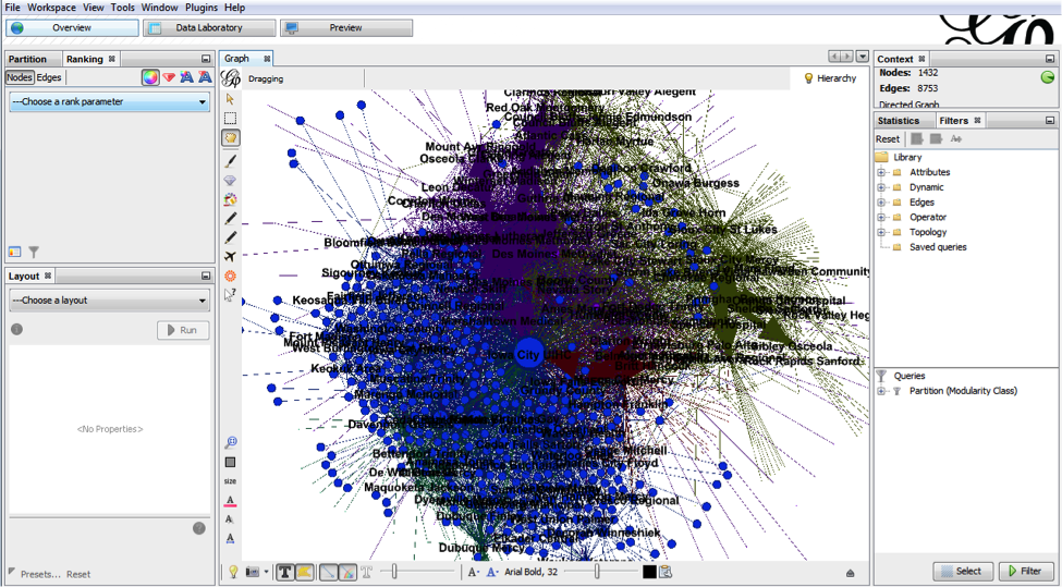
However, what most people want is to look at a graph of arbitrary size and understand things about the individual nodes.  When you do that you get something like this:


Labels overlapping labels, clusters of nodes where relationships are hidden.  Almost completely unusable.  There are some highly interconnected graph structures that look like this no matter how much you try to lay them out nicely.

It is, ultimately, extremely hard to get what people want from graph visualizations.  You can get it in special cases and with manual work per graph, but there is no general solution.

What's so hard about 3D data visualization?

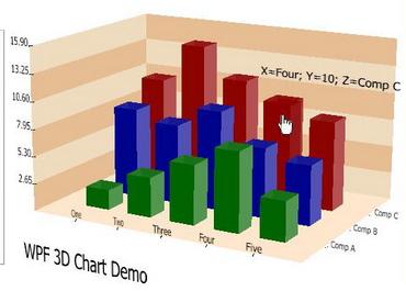
In theory, it seems like 3D should make visualization better.  It adds an entire dimension of data!  The reality is, however, we consume data in 2D.  Even in the physical world, a stack of 3D bars would be mostly useless.  The 3rd dimension tells us more about the shape of the first layer of objects in front of us.  It does not tell us anything about the next layer.  As such, visualizations like this are a 2D bar chart with clutter behind them:


Even when the data is not overlapping, placing the data in three dimensions is fundamentally difficult.  In the following example, it's almost impossible to tell which points have what values on what axes:

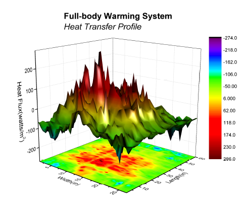
Granted, there are ways to help improve this, (mapping points to the bounding box planes, drawing lines directly down from the point to the x-y plane, etc), but in generally you would only do that if you _really_ needed that 3rd dimension (and didn't have a 4th).  Otherwise you might as well use PCA or such to project into a 2D plot.  Even a plot where the 3rd dimension provides some quick and easy insight, can practically be projected to a 2D heatmap:


Do you really need to visualize a graph?

Many times when people want to visualize a graph, what they really want is to visualize the data in the graph in the context of the edges.  Commonly, graph data can be subsetted with some type of graph transversal (e.g. [[select ip == xxx.xxx.xxx.xxx]] -> [[follow all domains]] <- [[return all ips]]) and the data returned in a tabular format.  This is usually the best approach if you are past a few dozen nodes. Even if long, this data can easily be interpreted as many types of figures (bar, line, point charts, heatmaps, etc).  Seeing the juxtaposition between visualizing graphs because they were graphs, but when the data desired was really tabular heavily influenced how I approached the problem.

My Attempt

First, I'll preface this by saying this is probably a bad data visualization.  I have few reasons to believe it's a good one.  Also, it is extremely rough; nothing more than a proof of concept. Still, I think it may hold promise.


The visualization is a ring of tiles.  Each tile can be considered to be a node.  We'll assume each node has a key, a value, and a score. There's no reason there couldn't be more or less data per node, but the score is important.  The score is "how relevant a given node is to a specified node in the graph.  This data is canned, but in an actual implementation, you might search for a node representing a domain or actor.  Each other  node in the graph would then be scored by relevance to that initial node.  If you would like ideas on how to do this, consider my VERUM talk at bsidesLV 2015. For now we could say it was simply the shortest path distance.

One problem with graphs is node text.  It tends to not fit on a node (which is normally drawn as a circle).  In this implementation, the text scrolls across the node rectangle allowing quick identification of the information and detailed consumption of the data by watching the node for a few seconds.  All without overlapping the other nodes in an illegible way.

Another problem is simply having two many nodes on screen at once time.  This is solved by only having a few nodes clearly visible at any given time (say the front 3x3 grid).  This leads to the question of how to access the rest of the data.  The answer is simply by spinning the cylinder.  The farther you get from node one (or key1 in the example), the less relevant the data.  In this way, the most relevant data is also presented first.

You might be asking how much data this can provide.  A quick look says there are only 12 columns in the cylinder resulting in 36 nodes, less than even the 60 we discussed above.  Here we use a little trick.  As nodes cross the centerline on the back side, they are actually replaced.  This is kind of like a dry-cleaning shop where you can see the front of the clothing rack, but it in fact extends way back into the store.  In this case, the rack extends as long as we need it to, always populated in both directions.

Demo


I highly recommend you try out the interactive demo above.  it is not pretty.  The data is a static json file, however that is just for simplicity.

Future Work

Obviously there's many things that can be done to improve it:
  • A search box can be added to the UI and a full back end API to populate the visualization from a graph.
  • Color can be added to identify something about the nodes such as their score relative to the search node or topic.
  • The spacing of the plane objects and camera can be adjusted.
  • Multiple cylinders could exist in a single space at the same time representing different searches.
  • The nodes could be interactive.
  • The visualizations could be located in VR or AR.
  • Nodes could be selected from a visualization and the sub-graph returned in a more manageable size (see the 60ish node limit above). These subgraphs could be stored as artifacts to come back to later.
  • The camera could be within the cylinder rather than outside of it.

Conclusion

I'll end the same way I began.  I have no reason to believe this is good.   It is, at least, an attempt to address issues in graph visualization.  I look forward to improving on it in the future.

Building a SEIM Dashboard with R, Jupyter, and Logstash/Elastic Search

Motivation:

I am disappointed with the dashboards offered by today's SEIMs.  SEIM dashboards offer limited data manipulation through immature, proprietary query languages and limited visualization options. Additionally, they tend to have proprietary data stores that limit expansion and evolution to what the vendor supports.  Maybe I'm spoiled by working in R and Rstudio for my analysis, but I think we can do better.

Plan:

This blog is mainly going to be technical steps vs a narrative.  It is also not the easiest solution.  The easiest solution would be to already have the ELK stack, install interact.io, R, the R libraries, and the R jupyter kernel on your favorite desktop, and connect.  That said, I'm going to walk through the more detailed approach below.  You can view the example notebook HERE.  Make sure to scroll down to the bottom where the figures are as it has a few long lists of fields.

Elastic search is becoming more common in security, (e.g. 1, e.g. 2).  Combine that with the elastic package for R, and that should bring all of the great R tools to our operational data.  Certainly we can create regular reports using Rmarkdown, but can we create a dashboard?  Turns out with Jupyter you can!  To test it out, I decided to stand up a Security Onion VM, install everything needed, and build a basic dashboard to demonstrate the concept.

Process:

Install security onion:

Security onion has an EXCELLENT install process.  Simply follow that.

Install R:


Added ‘deb https://mirrors.nics.utk.edu/cran/bin/linux/ubuntu trusty/‘ to packages list

sudo apt-get install r-base

sudo apt-get install r-base-dev

— based off r-project.org

Install R-studio (not really necessary but not a bad idea)


Downloaded r-studio package from R-studio and installed

Sudo apt-get install libjpeg62

sudo dpkg -I package.deb

Install Jupiter:


(https://www.digitalocean.com/community/tutorials/how-to-set-up-a-jupyter-notebook-to-run-ipython-on-ubuntu-16-04)

Sudo apt-get install python-pip

sudo pip install —upgrade pip (required to avoid errors)

sudo -H pip install jupyter 

Install Jupyterlab: (probably not necessary)


Sudo -H pip install jupyterlab

Sudo jupyter serverextension enable --py jupyterlab --sys-prefix

Install Jupiter dashboard

(https://github.com/jupyter/dashboards)

sudo -H pip install jupyter_dashboards

sudo -H pip install --upgrade six

Sudo jupyter dashboards quick-setup --sys-prefix 

Install R packages & Jupypter R kernel:

Sudo apt-get install libcurl4-openssl-dev

sudo apt-get install libxml2-dev

Start R

install.packages("devtools") # (to install other stuff)

install.packages(“elastic”) # talk to elastic search

install.packages(“tidyverse”) # makes R easier

install.packages("lubridate") # helps with working with dates

install.packages("ggthemes") # has good discrete color palettes

install.packages("viridis") # has great continuous colors

# https://github.com/IRkernel/IRkernel

devtools::install_github('IRkernel/IRkernel')

# or devtools::install_local('IRkernel-master.tar.gz')

IRkernel::installspec() # to register the kernel in the current R installation

quit() # leave. Answer ’n’ to the question “save workspace?”

Install nteract: (Not necessary)

(nteract.io)

Download the package

Sudo apt-get install libappindicator1 libdbusmenu-gtk4 libindicator7

sudo dpkg -i nteract_0.2.0_amd64.deb


Set up the notebook:

Rather than type this all out, you can download an example notebook.  In case you don't have an ES server populated with data, you can download this R data file which is a day of windows and linux server logs queried from ES from a blue vs red CTF.

I created the notebook using nteract.io so it is in a single order.  However, if you open it on the juypter server, you can use the dashboards plugin to place the cells where you want them in a dashboard.

Results:

A lot of time spent compiling.

No need to download R/jupyter stuff on security onion if elastic search is remotely reachable.

Elastic search is not intuitive to query.  Allowing people an 'easy mode' to generate queries would be significantly helpful.  the `ES()` function in the workblook is an attempt to do so.

It would be nice to be able to mix interactive and dashboard cells.

This brings MUCH more power for both analysis _and_ visualization to the dashboard.

This brings portability, maintainability (ipynb files can be opened anywhere that has the R/jupyter environment and can access elastic search.  They can also be forked, version controlled, etc.)

Future Work:

Need a way to have cells refresh every few minutes, likely a jupyter notebook plugin.

Interactive figures require interactive plotting tools such as Vega.  This would also bring the potential ability to stream data directly to the notebook.  It may even solve the ability to auto-refresh.

Conclusion:

In conclusion, you really don't want to roll-your-own-SEIM.  That said, if you already have ES (or another data store R can talk to) in your SEIM and want less lock-in/more analysis flexibility, R + Jupyter may be a fun way to get that extra little emph.  And hopefully in the future we'll see SEIM vendors supporting general data science tools (such as R or Python) in their query bars and figure grammars (ggplot, vega, vegalite), in their dashboards.